Please put it on the Map and see how far it falls from mine.
1 Thank
Done. Looks like my estimate has more output and less throw.
ZeroAir’s M21J numbers are 3426lm and 794m, less output and more throw compared to PTD’s numbers I used. If I use ZeroAir’s numbers, I’d say 4800lm and 560m instead. Since ZeroAir’s measurement distances are short and favor flooders, I’d guess that he could measure 600m. Let’s see who reviews it first!
1 Thank
There is a different idea that I would like to check. Knowing the Acuity Index, what’s the beam divergence angle estimate?
I cooked this formula (based on beam limits being FWHM intensity, Gaussian radial distribution within the beam, and f fraction of total lumens going into the beam which depends on 1 - spill angle and thus the h/D of the reflector):
beam divergence angle = [360/pi*sqrt(ln(2))*sqrt(f)]/Acuity_Index
If I fix f at around 0.8 for reflectors close to h/D=1, it simplifies to:
~85/Acuity_Index
Would it pass sanity test, I wonder?
Could you elaborate on how Gaussian distribution and ln(2) come in? I find Gaussian to be a weird model for angular distribution, since the Gaussian has unbounded support, but angular distribution is over a bounded domain.
Anyways, I tried to derive a formula assuming that all of the light goes into either the hotspot of the spill, i.e., no corona. The resulting formula I got for the diametrical angle was
360/pi sqrt(f)/a,
where a is acuity index. For f=0.8, this becomes 102.5/a, which is known to be an overestimate because in reality some of the hotspot is diverted into the corona. So I’d say that the coefficient of around 85 is reasonable, with the underlying correction factor being sqrt(ln 2)=0.83. The question is, how did you get the ln(2) in there?
It’s a bit messy and I need to go over it again to convince myself, but you assume the beam intensity to be unbounded Gaussian (radially from the peak on the axis) for the fraction of output feeding the beam (another integration) then you truncate the tails at FWHM (beam boundary as we see it definition). Then when you solve for the angle at FWHM you end up with an expression involving √(2ln(2)) - a consequence of exp() in the Gaussian PDF. In the end several terms cancel out and you’re left with the above (I hope).
The choice of Gaussian is arbitrary (one could fiddle with the Central Limit Theorem to justify it, I suppose), but it helps in this canceling out above. All I know is that the beam intensity distribution is peaky not flat and employing Gaussian to describe it is probably super good enough.
1 Thank
Got it, thanks for the explanation! I see that you defined the hotspot to be the half-intensity cutoff, which is probably a good definition to use.
I tried an alternate derivation via ray tracing, and ended up with a formula that suggests a tighter hotspot than yours. Could you take a look and see if it seems sensible?
A nice surprise is that the “beam acuity index” happens to be a very convenient quantity to work with throughout the derivation.
1 Thank
A new plot showing the relative hotspot sizes (at fixed distance, or equivalently the hotspot full angle) has been added to the Map of Flashlights. You can hover on the interactive version to get more numerical specs.
Please take a look and let me know if it makes sense.
4 Thanks
Very interesting idea. Thanks.
3 Thanks
@koef3: are real bare LEDs anywhere close to Lambertian emitters?
1 Thank
Yes, this should also apply to those with dome. There are some LEDs with “3D” LES (older XT-E, see image of LED in this datasheet) which have different spatial distribution.
3 Thanks
Many thanks for reviewing the model.
I have modified the model and its description since. Please take another look, especially the section on Super-Gaussian and choices of parameters and their consequences.
I think the formulation used in the model may be correct and there is no inconsistency.
The regular 1-D Gaussian (1-D because the support is a line) applies to the axial section of the beam. 2.35 ≈ 2×1.1774 comes from the FWHM being full width on both sides of the axis. The area under such PDF curve between FWHM limits would be some 76% of the total. This has nothing to do with beam dimensionality.
If you rotate such distribution around its axis, that becomes 2-D isotropic Gaussian (now the support is a plane). I think that one of the fancy names for it is bivariate Gaussian/Normal with equal variance and zero covariance.
The angular intensity distribution is still 1-D Gaussian as before, but now to get the portion of the flux contained in the beam cone (or greater than half max intensity), you need to find the volume under the surface, not the area under the curve.
For the rotated Gaussian this volume has a nice property: For FWHM limits, 50% of the volume (flux) is in the hotspot and 50% outside it. For more general FWpM limits 1-p fraction of the flux is contained within the hotspot. This does not hold for Super-Gaussian and you need to integrate to get it. The model description has a bit more on that.
Many thanks for the clarifications! The super-Gaussian distribution at a first glance seems to model the beam better than the standard Gaussian, though I need to spend more time studying it. The rapidly-decaying tails, like the Gaussian distribution, make it unsuitable for modeling spill.
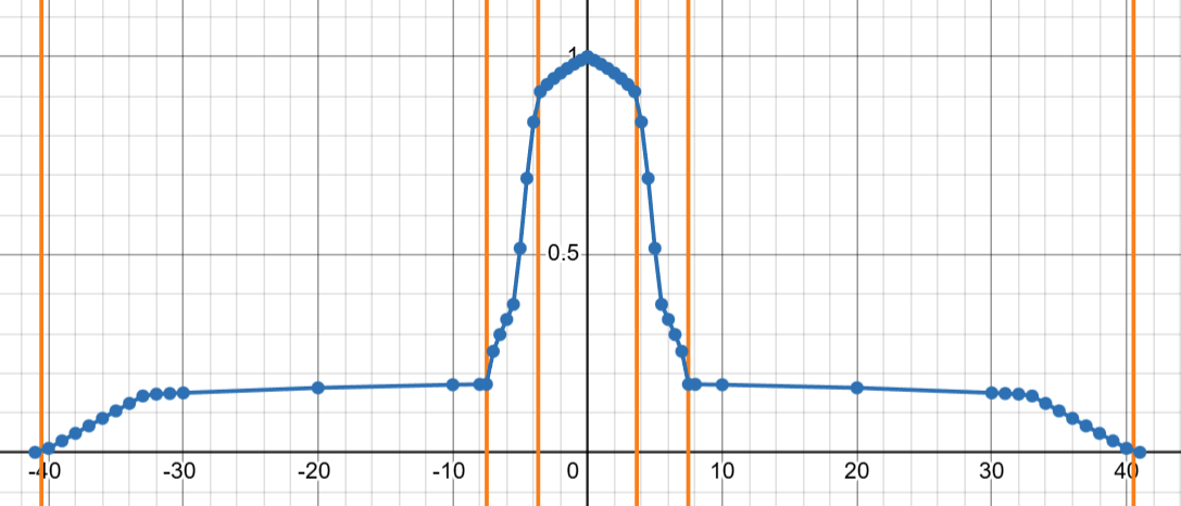
Here’s the angular intensity plot I got from simulating a S2+ SFT42R, but in 2D. The 3D version can be expected to have a greater intensity ratio between hotspot and spill, plus slightly smoother transitions between them.
Also, you mention that
Could you share the explicit measurements?
[EDIT: did the math and ~2.35 is the correct diametrical angle for the 50% total flux cutoff. It appears that the disagreement here is not mathematical in nature, but caused by imprecise communication.]
I think that’s where the issue is. A 2D Gaussian has coordinate marginals that are 1D Gaussian, but the distribution of radius is no longer Gaussian or half-Gaussian.
The standard 2D Gaussian has density 1/(2π) e^{-(x^2+y^2)/2}, which is expressible as 1/(2π) e^{-r^2/2}. To get from point density to radial density, you need to multiply by a factor of 2πr (i.e., circumference), to get re^{-r^2/2}, because going from 2D space to one-dimensional radius-space involves collapsing circles around the origin into points in radius-space, so points in radius-space need to inherit the mass of the entire circle it used to be.
Another way to see this is via polar integration of the density, which gives you
\int_{θ=0}^{2π} \int_{r=0}^{R} 1/(2π) e^{-r^2/2} r dr dθ = \int_{r=0}^{R} e^{-r^2/2} r dr.
A few bug fixes and improvements to the Map of Flashlights.
The most significant one is that now the relative diameters of the circles on the Hotspot Size plot correlate better with what to roughly expect in reality.
Hovering on the lights pops up more numerical specs.
Also discovered this wonderful creation by @grzybek337 that goes well with the Map:
1 Thank